
If you think this is controversial, this is the blog for you.
Heads up: This blog relates to statistical analysis and is a bit more technical than our regular blogs. We hope you enjoy deep diving into this debate.
What is a binary outcome?
When working in behavioural insights, the outcome we want to change is often measured with a binary variable. Binary outcomes are events with only two possible values, like whether someone submitted a tax return or not. When we model these outcomes, we usually include the two categories as ones and zeros where 1 = the target outcome (i.e. submitting their tax return) and 0 = not the target outcome (i.e. not submitting their tax return).
When linear regressions and binary outcomes don’t mix
If you’ve done some undergraduate statistics, you’ll probably remember being told not to use linear regression to model binary outcomes to predict the probability of something happening.
For example, imagine we wished to predict the probability of passing a test based on age. Generally, when people get older they have a higher chance of passing this test. Age is a continuous variable, which means that it has ‘infinite’ different values which we are modelling, i.e. age can be equal to 10, 11, 11.3, 25.7.
If we use a linear model, we can have high values that result in probabilities greater than 1. For instance, let’s say that for every additional year of age over 13, a person has a 30% higher chance of passing the test (i.e. the coefficient for age is 0.30). If someone is aged 18, then they have a 150% (5 x 0.33 = 1.5) chance of passing the test! This does not make any sense.
The figures below show why you’ve been told to only use linear models for continuous variables.
Figure 1 shows a linear relationship between a continuous x variable (e.g. age) and a continuous y variable (e.g. weight). The line fits the data well.
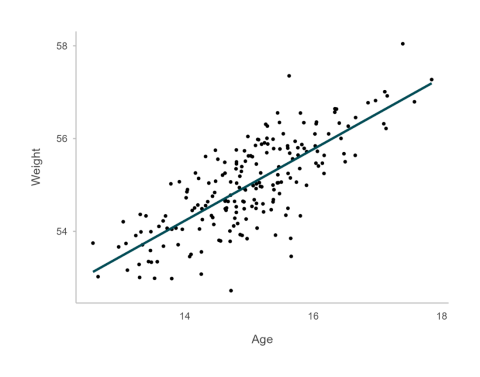
Figure 1
In Figure 2, we see a line trying to describe a relationship between a linear x variable (e.g. age) and binary y variable (e.g. passing a test). As you can see, a linear model does not represent the relationship well. Instead, to model this type of relationship we usually use a model called a logistic regression or logit.
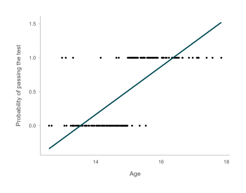
Figure 2
The logit model, shown in Figure 3, takes into account the shape of the binary y variable plotted with a continuous x variable and constrains the probabilities to between 0 and 1.
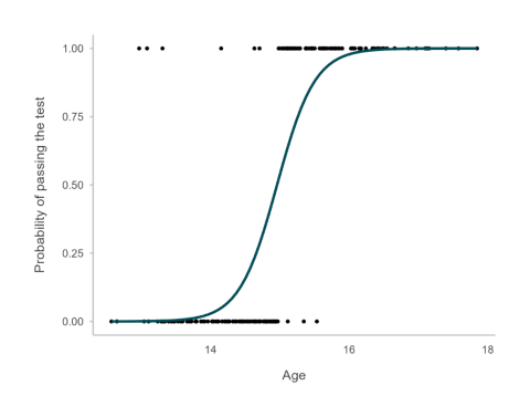
Figure 3
Why randomised controlled trials are different
Unlike the example above where you’re trying to predict the probability of something happening (e.g. passing a test), in behavioural insights we often aren’t trying to predict anything: instead we are trying to estimate the impact of an intervention using a randomised controlled trial. The crucial difference here is that our predictor is also a binary variable – treatment assignment.
Imagine that our trial separated students into two groups at random where one group received a new program (treatment group) and one received the usual program (control group). To test whether the new program was better than the usual program, we compare the rate of students who pass in each group (this would be coded as fail = 0, pass = 1).
Now, instead of predicting a pass based on something like age, we are estimating the difference between two groups. This difference is a proportion of passes in each group or simply a group mean. We can use a linear regression model called ordinary least squares (OLS) for this without generating values that don’t make sense. When we use OLS for our binary outcomes in randomised trials, we call it a linear probability model (LPM).
Benefits of using Linear Probability Models
There are some big benefits to using LPMs in your randomised trials with binary outcomes.
First, the coefficient for the treatment effect can be directly interpreted. Say we have a behavioural intervention to increase enrolments in a course. A coefficient of 0.07 means that there was a 7 percentage point difference in the probability of enrolment between the treatment and control groups. Compare this to the logit model where the coefficient is the expected change in log odds between treatment and control. This is extremely hard to interpret or explain and beyond the scope of this blog.
Second, statisticians tested the accuracy of LPMs versus logit models and found that LPMs can provide more accurate results. Using a logit model may result in artificially small standard errors, which can lead to false positive results, where you think there was an effect of your intervention but there actually wasn’t.
Addressing some common concerns
You may have some concerns that might come to mind here. Sometimes, people are concerned because they have a continuous covariate in their model, like age. With a binary outcome and continuous predictor, aren’t we back in a world of pain with misspecified models? The answer is no, because we are running a randomised controlled trial. This means:
- We don’t care about the coefficients for the covariates as they are not what we are estimating. We are only interested in the coefficient for the treatment variable.
- Covariates are uncorrelated with treatment, since treatment is assigned at random. This means the estimated impact of treatment is unbiased even if we have continuous covariates.
The second common concern is around heteroscedasticity. OLS model has an assumption of homoscedasticity, which is when the variance of the residuals is equal over the range of measured values. When this assumption is violated it is termed heteroscedasticity. The LPM will violate this assumption. However, we can manage this easily by using robust standard errors in our regression model.
So, what should you take away from this?
If you are predicting the probability of events based on modelling, like we did when using age to predict probability of passing a test, you should stick with what you were taught at uni and not use the linear probability model.
However, if you are running randomised trials, the linear probability model is your friend. It is easier to interpret, easier to run, easier to explain and more accurate. At BETA we use the linear probability model with robust standard errors as our primary estimator and you should too.
Further reading
- Deke J (2014) Using the linear probability model to estimate impacts on binary outcomes in randomized controlled trials. Evaluation Technical Assistance Brief, number 6, Office of Adolescent Health (PDF 1.1MB)
- Gomila R (2021) Logistic or linear? Estimating causal effects of experimental treatments on binary outcomes using regression analysis. Journal of Experimental Psychology: General, 150(4): 700-709. DOI: 10.1037/xge0000920.